

Air Quality—Meteorology Correlation Modeling Using Random Forest and Neural Network
by
Ruifang Liu
1,2,*,
Lixia Pang
3,
Yidian Yang
1,
Yuxing Gao
1,
Bei Gao
4,
Feng Liu
1 and
Li Wang
1 1
Xi’an Meteorological Observatory, Xi’an 710016, China
2
Key Laboratory of Eco-Environment and Meteorology for the Qinling Mountains and Loess Plateau, Xi’an 710016, China
3
Nanjing University of Information Science and Technology, Nanjing 210014, China
4
Shaanxi Meteorological Service Center of Agricultural Remote Sensing and Economic Crops, Xi’an 710014, China
*
Author to whom correspondence should be addressed.
Sustainability 2023, 15(5), 4531; https://doi.org/10.3390/su15054531
Submission received: 29 November 2022
/
Revised: 17 February 2023
/
Accepted: 17 February 2023
/
Published: 3 March 2023
(This article belongs to the Special Issue Soil-Water-Plants and Environmental Nexus)
Abstract
:Under the global warming trend, the diffusion of air pollutants has intensified, causing extremely serious environmental problems. In order to improve the air quality–meteorology correlation model’s prediction accuracy, this work focuses on the management strategy of the environmental ecosystem under the Artificial Intelligence (AI) algorithm and explores the correlation between air quality and meteorology. Xi’an city is selected as an example. Then, the theoretical knowledge is explained for Random Forest (RF), Backpropagation Neural Network (BPNN), and Genetic Algorithm (GA) in AI. Finally, GA is used to optimize and predict the weights and thresholds of the BPNN. Further, a fusion model of RF + BP + GA is proposed to predict the air quality and meteorology correlation. The proposed air quality–meteorology correlation model is applied to forest ecosystem management. Experimental analysis reveals that average temperature positively correlates with Air Quality Index (AQI), while relative humidity and wind speed negatively correlate with AQI. Moreover, the proposed RF + BP + GA model’s prediction error for AQI is not more than 0.32, showing an excellently fitting effect with the actual value. The air-quality prediction effect of the meteorological correlation model using RF is slightly lower than the real measured value. The prediction effect of the BP–GA model is slightly higher than the real measured value. The prediction effect of the air quality–meteorology correlation model combining RF and BP–GA is the closest to the real measured value. It shows that the air quality–meteorology correlation model using the fusion model of RF and BP–GA can predict AQI with the utmost accuracy. This work provides a research reference regarding the AQI value of the correlation model of air quality and meteorology and provides data support for the analysis of air quality problems.
1. Introduction
In recent years, China’s economy has developed rapidly and made remarkable achievements. Subsequent environmental problems, such as Air Pollution (AP), have also attracted public attention [1]. The research demonstrates that China’s spatial distribution, seasonal variation, and interannual air quality vary greatly. From the perspective of spatial distribution, the national air quality shows an obvious spatial agglomeration law and differentiation. It manifests in the spatial pattern of heavier pollution in the north and east with better air quality in the south and west. For example, the air pollution in Beijing, Tianjin, Hebei, and surrounding areas is relatively high. The southern coastal areas, such as the Pearl River Delta, and western regions, like the Yunnan Guizhou Plateau and the Qinghai Tibet Plateau (QTP), mostly enjoy excellent weather throughout the year. From the viewpoint of seasonal changes, the air quality is generally good in summer, followed by spring and autumn, and poor in winter, with heavy pollution weather occurring frequently. From the perspective of monthly distribution, the national and regional air quality present a U-shaped change pattern. There is low pollution in summer and high pollution in winter, with falling pollution in spring and rising in autumn [2,3]. Thus, improving air quality is urgent for dealing with serious AP. In 2013, the State Council of China issued the Air Pollution Prevention and Control Action Plan. From the point of interannual changes, air quality has steadily improved in recent years [4]. From 2013 to 2017, the average concentration of PM (Particulate matter) 2.5 () in Beijing, Tianjin, Hebei, the Yangtze River Delta, and the Pearl River Delta decreased by 37%, 34%, and 28%, respectively. This index exceeded the set air-quality improvement target [5]. In 2021, the national ecological environment quality was significantly improved. However, the inflection point of the ecological environment quality from a quantitative to a qualitative change has not yet appeared. The overall urban ambient air quality has not reduced the meteorological impact [6]. That is, the air quality of a region is greatly affected by meteorological conditions. When meteorological conditions are conducive to the diffusion of air pollutants, the air quality is relatively good, whereas when meteorological conditions are not conducive to the diffusion of pollutants, the air quality worsens significantly. Meteorological conditions will have a short-term impact, resulting in heavy pollution. Meanwhile, they have a long-term impact on air quality, resulting in precipitation decreases, wind direction variation, or air quality recovery [7,8,9,10,11].
Forest meteorological environment data are an important basis for understanding the forest system and also the basis for studying and protecting the forest system. With the development of science and technology, the observation of forest meteorological environments is increasingly dependent on automatic monitoring and technology. The designed air quality–meteorology correlation model is automatic weather station equipment based on the Internet of Things, big data, data analysis, and other new-generation information technology. Using various sensors to automatically acquire the weather, the system realizes information management, intelligent monitoring, and automatic integrated real-time monitoring of meteorological data. It helps forest managers timely obtain meteorological data, conduct online statistical analysis, and take effective early warning and preventive measures to protect forest environmental security.
The air quality–meteorology correlation model can greatly improve the timeliness and effectiveness of forest meteorological data observation in forest ecosystem management and help relevant personnel to understand forest meteorological dynamics in a timely manner. Moreover, these meteorological environmental data can also be used for statistical analysis and prediction of forest ecological conditions, thus guiding forest production and management and preventing forest disasters. In forest ecosystem management, the air quality–meteorology correlation model can be used for forest meteorological and ecological environment monitoring; meteorological monitoring of planting plants; conventional meteorological monitoring of field ecological stations; conventional monitoring of the water cycle, heat balance, carbon cycle, and other research topics; regional water monitoring; provincial, municipal, and county meteorological monitoring networks; meteorological monitoring of tourism suitability indices of parks and scenic spots; and forest fire prevention. It plays a crucial part in intelligent meteorological services in many fields.
During the global warming process, the total forest productivity in China shows an increasing tendency, which is affected by the rising temperature and precipitation. Nevertheless, in the future, as global warming further intensifies and local drought intensifies, total productivity will stop growing or even show negative growth. According to the 2021 Climate Blue Book, China’s average temperature has risen by 1.5 °C in the past 60 years. This rise is significantly higher than the global average level in the same period. The temperature rise is distributed in the central and northern northeast and central northwest regions. In particular, inner Mongolia and northwest Tibet have had the highest average warming (2.0–3.0 °C), followed by North China, eastern coastal areas, and central Xinjiang (1.0–2.0 °C). The lowest temperature (0–1.0 °C) was found in western central China, western South China, and southwest China. When global warming reaches 1.5 °C, the promoting effect of temperature on forests in the Greater Khingan Mountains will disappear, and the total productivity will decrease as a result of drought and fire. Seasonal drought across regions increases forest mortality risk and limits forest productivity growth. Climate change has also given rise to extreme natural events, such as fires, pests and diseases, hurricanes, and an increased risk of forest degradation and mortality. Climate change is a major challenge worldwide. Thus, curbing climate change requires the joint efforts of all humanity. Forests are powerful carbon sinks. Vigorously carrying out afforestation can effectively mitigate climate change and enable people to participate in combating climate change.
Random Forest (RF) is mainly used for regression and classification. RF algorithms have been applied in various fields by many scholars in and out of China. In the field of image science, image processing research for a large number of scenes includes image recognition and classification, target detection, and other subdivision directions [12]. Of these, image processing segments large images into small images. Through pixelization, a single image is divided into multiple small-pixel images, thus developing into a classification problem. In terms of genetics, for massive gene data, high dimensionality leads to a low recognition ability of disease genes using traditional data analysis methods [13]. Some scholars use RF algorithms to study gene recognition and protein interaction. In the financial field, the RF algorithm plays an important role in image recognition, anomaly detection, and text classification [14].
AP is closely related to the type, distribution, meteorological conditions, and topography of pollution sources. However, due to a specific area’s landform and pollution source conditions being relatively stable within a certain time range, geographical environment, economic environment, and meteorological conditions are the key to determining the concentration distribution of urban air pollutants. Many scholars have studied the relationship between air pollutants and meteorological conditions. Lolli et al. [15] analyzed the relationship between main pollutants and meteorological conditions and found that the northwest wind was more conducive to the diffusion of pollutants in cities, and precipitation, relative humidity, and wind speed have a significant impact on air quality. Ceylan et al. [16] used the Pearson Correlation Coefficient (PCC) and Spearman Correlation Coefficient (SCC) to analyze the correlation between environmental factors, such as temperature, humidity, and air quality. The research results showed that environmental factors impacted air quality. Zhou et al. [17] studied the impact of waste and industrial pollutants on developing nations’ air quality and revealed that industrial waste was a primary cause of air pollution. Gan et al. [18] used correlation analysis to analyze the correlation between automobile waste emissions, industrial construction, industrial development, and urban green land occupation. They found that industrial waste contributed most significantly to air pollution. In the research on Machine Learning (ML) and air quality, Shahriar et al. [19] predicted PM 2.5 in the air through Decision Tree (DT) and Support Vector Machine (SVM) model. The prediction results were affected by the concentration of PM 2.5 and meteorological conditions such as precipitation and wind speed. The research showed that DT and SVM models could forecast the concentration of PM 2.5 in the air. Gocheva-Ilieva et al. [20] predicted the air quality through Random Forest (RF), SVM, and Classification and Expression Tree (CART) model. They compared and analyzed the prediction performance of three ML algorithms and discovered that the RF algorithm was the most accurate in predicting meteorological factors and air pollutants. Menéndez García et al. [21] designed an RF model to forecast the air quality of Swiss meteorological factors and air pollutants. They proved that RF had excellent accuracy in air quality prediction. Liu et al. [22] used a Backpropagation Neural Network (BPNN) learning algorithm to predict air quality in Greece. The research showed that the BP-predicted value was very close to the actual air-quality detection value. Li et al. [23] devised BPNN and Long Short-Term Memory (LSTM) models to forecast air quality in Poland and India. The results indicated that BPNN and LSTM models could accurately forecast regional air quality.
Ogeneovo et al. [24] applied an ID3 (Iterative Dichotomizer 3) DT algorithm to environmental monitoring data and achieved good results. Althuwaynee et al. [25], using the DT algorithm, selected two combined attributes in the test attribute similarity as the information-gain correction factor for calculating air quality to evaluate air quality. Singh et al. [26] used the Support Vector Machine (SVM) to classify and predict major urban environmental data in China. Eldakhly et al. [27] used grey theory and SVM to predict PM 2.5 concentration. Jiang et al. [28] carried out parameter optimization and model improvement on the SVM algorithm and improved the air quality early warning model based on a combination algorithm and Particle Swarm Optimization (PSO) to make the improved algorithm evaluation results more accurate. Bai et al. [29] applied the rough set method to air quality evaluation and extracted its rules. The research results showed that rough set theory was an effective tool for knowledge reasoning and expert system establishment.
According to the above scholars’ findings, there are correlations between air quality and meteorological conditions, air pollutants, and industrial development. The impact of industrial waste emissions on air quality or environmental factors on air quality all involve studying the change process of air quality. At the same time, RF and neural network models have successfully lent to air quality predictions [30]. The results provide methodological guidance for exploring the air quality–meteorology correlation model. However, the prediction accuracy of the traditional single-term algorithm for nonlinear air quality data is not high, and the model’s generalization ability is weak. For high-dimensional data, it is easy to cause modeling failure, so the air quality–meteorology correlation model cannot be fully analyzed, resulting in low model performance. The research results show that both RF and NN models successfully predicted the air quality model. Hence, the ML algorithm will be integrated to establish the air quality–meteorology correlation model. The ML algorithm can process high-dimensional data without feature screening and with high prediction accuracy, good generalization ability, and strong anti-interference ability. When missing values exist in the data, the prediction accuracy can still be maintained.
A high-accuracy air quality–meteorology correlation model is obtained while providing a survival guarantee for forest ecosystem species and implementation strategies for forest ecosystem management. Firstly, this work discusses the related theory of RF and BPNN models and uses a Genetic Algorithm (GA) to optimize and forecast the weight and threshold of BPNN. Therefore, the effects of climate change on the forest ecosystem are illustrated. Finally, the impact of meteorological conditions, such as temperature, humidity, and wind level, on air quality is analyzed. Some suggestions of sustainable development management strategies for forest ecosystems under climate change are also put forward. The AQI results of the RF and Backpropagation–Genetic Algorithm (BP–GA) models are analyzed. The RF algorithm, BPNN model, and GA are combined, and the GA is used to optimize the prediction of the network weights and thresholds in the BPNN, reducing the dimension of the input factors, reducing the interference of irrelevant dimensions, and realizing the optimization of the urban air quality–meteorology correlation model. This work’s proposed model is different from the previous fusion model for air quality prediction. On the one hand, it improves the prediction accuracy and provides research references for AQI prediction using the air quality–meteorology correlation model. On the other hand, it combines meteorology and air quality factors to carry out fusion model prediction, which provides data support for the analysis of air quality problems. This innovation puts forward the concept of the RF + BP + GA fusion model and establishes a feature selection method suitable for evaluating the air quality–meteorology correlation model. This research surpasses air quality prediction that uses a traditional single algorithm. The combined prediction model of RF, neural network, and GA is used to predict air quality with higher prediction accuracy. It can not only predict the AQI but also provide an implementation strategy basis for forest ecosystem management.
This work is divided into five parts. Section 1, the introduction, mainly describes the research background; the research on the relationship between the air quality model, meteorological conditions, and machine learning conducted by domestic and foreign scholars; and explains the necessity of this research. Finally, it describes the research method’s process, significance, innovation, and framework. Section 2, regarding the research methods, mainly introduces the theory of the RF algorithm, BP algorithm, and GA. An air quality and meteorology correlation fusion model based on RF + BP + GA is proposed to explain the role of forests in climate regulation and the source of the experimental data of this work. Section 3 analyzes the research results from the perspective of the changing trend of AQI and meteorological conditions and the interaction between the climate conditions correlation model and the forest ecosystem. Section 4 is the conclusion, including the research results, research significance, and future prospects.
2. Materials and Methods
2.1. Experimental Data
Pollutant emissions will not change greatly in the short term for a particular area. However, the ambient air quality will change considerably. The monitoring results of pollutant concentrations from the same emission source at the same place are not necessarily the same. Sometimes, a very high concentration can be measured, and sometimes, a shallow concentration can be measured, with significant differences. The main reason for this change is a change in weather conditions: the ability of atmospheric transportation, dilution, transformation, and removal of pollutants has changed [31]. The migration and diffusion laws of pollutants vary according to different meteorological conditions. This section collects the air quality of Xi’an in Shaanxi Province and uses the real-time air quality detection data from Xi’an from 24 to 30 June 2022 as research data. The data from 18 June 2022 to 24 June 2022, are used to predict the AQI. The data comes from the Air Quality Implementation and Release System in Shaanxi Province.
AQIs can describe the air quality within the new ambient air quality standard. Common AQIs include the Air Pollution Index (API), Oak Ridge Air Quality Index (ORAQI), Extreme Value Index (EVI), and Pollutant Standard Index (PSI) [32,33]. Table 1 exhibits the applicable range of different evaluation indices.
According to the evaluation scope and applicable range of different evaluation indices in Table 1, AQI is selected to evaluate the air quality–meteorology correlation model in Xi’an. AQI is dimensionless and quantitatively describes air quality. Air-quality evaluation mainly involves six pollutants: fine particles, inhalable particles, sulfur dioxide, nitrogen dioxide, ozone, and carbon monoxide [34]. Equation (1) gives the specific calculation:
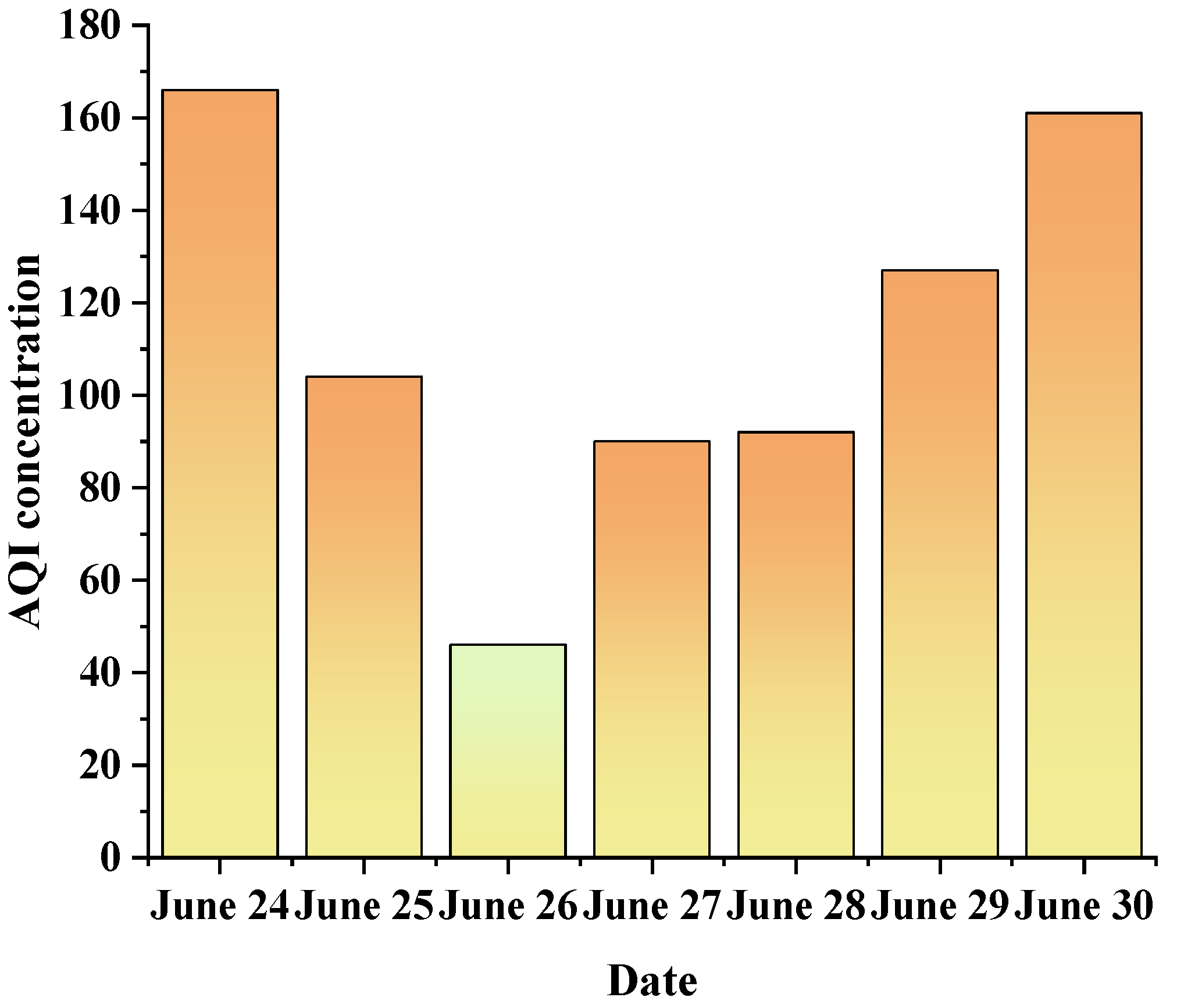
In Equation (1), refers to the air quality subindex of pollutant project . is the mass concentration of pollutant item . represents the air quality subindex of the corresponding area and the concentration index of the corresponding pollutant project. indicates the air quality subindex and the corresponding pollutant project concentration index of the corresponding region. means the air quality subindex of the corresponding region and the corresponding pollutant project concentration index. stands for the air quality subindex of the corresponding region and the corresponding pollutant project concentration index. Secondly, the maximum value of for various pollutants is selected and determined as AQI. When AQI > 50, the pollutant with the largest is determined as the primary pollutant [35]. Figure 1 illustrates the changes in the AQI index value in Xi’an from 24 to 30 June 2022.
In Figure 1, Xi’an had the lowest AQI and the best air quality on 26 June 2022. Except for 26 June 2022, Xi’an had certain air quality issues that week. The AQI on 24 and 30 June was the highest, reaching 166 and 161, respectively. Therefore, the air pollution in Xi’an is still serious. Most of the time, the air is polluted. The analysis indicates that such air quality is related to the continuous high temperature in Xi’an since June. The continuous high temperature changes the proportion of fine particles, inhalable particles, sulfur dioxide, nitrogen dioxide, ozone, and carbon monoxide in the air.
2.2. Random Forest (RF) Algorithm Theory
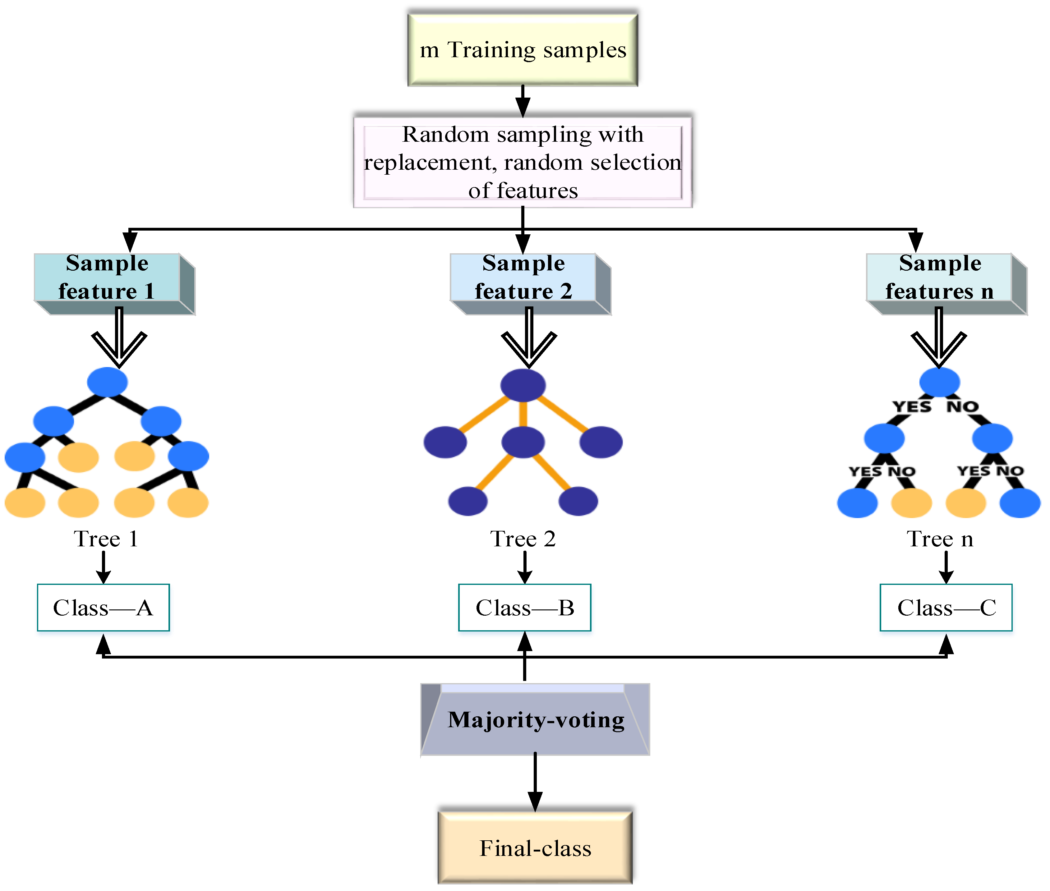
An RF is a forest constructed in a random way and consists of many DTs. The DTs in an RF are independent of each other. After the forest training, when there is new data input, all the DTs in the RF are calculated independently. For the classification problem, the prediction result is determined by calculating the votes of the DT; For he regression problems, the evaluation average of all DT prediction results is usually calculated as the final RF prediction results. This method is advanced because of the random selection of features of the RF on the basis of random sampling of Bagging samples. The basic idea is within the scope of Bagging [36]. Figure 2 details the basic principle of an RF.
In Figure 2, the RF builds forest randomly. Multiple DTs exist independently in the forest. Each of these DTs judges every new input of the RF to calculate which class is selected the most. Then, the class the sample belongs to is forecasted. Importantly, sampling and total splitting are the two crucial processes in building a DT. First, the RF uses two instances of random sampling to sample the rows and columns of input data. The putting-back method is adopted for row sampling. Thus, duplicate samples may be in the sample set. It is assumed that there are input samples. Then, samples are sampled. In this way, each DT does not input all samples during training, thereby avoiding overfitting. Second, column sampling is performed, and features are selected from features. The DT is established by completely splitting the sampling data until any leaf node cannot be further split or all samples in the leaf node point to the same category. The first two random sampling processes ensure that randomness and fitting do not occur even without pruning when the number of layers is small [37,38]. In DT-based classification, information gain can eliminate random uncertainty. Equation (2) expresses the information quantity:
In Equation (2), represents the event set. is the event category of . denotes the amount of information. indicates the probability of occurrence of . and are proportional. The expected value of the variable is calculated with entropy. Equations (3) and (4) calculate the information entropy:
In Equations (3) and (4), represents the conditional entropy of random variable under condition . is the information entropy of the random variable . This work chooses the C4.5 to calculate the DT-based classification or regression problems and uses Information Gain Ratio (IGR) to select attributes. The specific calculation reads:
Here, is the gain measure. represents the split information measure. denotes the sample subset formed by the values of . means the sample attribute. The classification results of the established RF are calculated with Equation (8):
In Equation (8), represents the final model of the RF. is the DT classification model, which can be C4.5 or CART algorithms. denotes the classification model of each DT, and stands for the classification result of . The RF can process very high-dimensional data (with many features). After the training, the RF can output the importance of features. Figure 3 displays the importance of sample features in RF training.
Figure 3 has four sample features: , , , and . Suppose feature is replaced by noise , and modeling is carried out accordingly. When the difference between the classification error rates Error 1 and Error 2 is small, the importance of feature is low. When Error 2 is much larger than Error 1, it means that the feature has a greater impact on the classification results. Table 2 lists the algorithm flow of the RF:
2.3. Theoretical Knowledge of the BP–GA NN
A BPNN is mainly composed of forward propagation and backpropagation. The network with n input nodes and m output nodes is regarded as a mapping of an n-dimensional Euclidean space. Through the principle of least squares and gradient search technology, the weights and thresholds are constantly learned and adjusted. If the output of the output layer is significantly different from the expected value, the error signal is sent back to each network layer unit of the network, and the mean square error between the actual output and the expected output of the network is minimized by modifying the weight and threshold of each layer neuron. The BPNN is a Multilayer Feedforward Neural Network (MLFNN) with some unique characteristics: the neurons of each layer are completely interconnected with the neurons of the next layer. No same-layer neuron connections exist. No cross-layer neuron connections exist [39]. Figure 4 presents the connection structure between BPNN neurons.
According to Figure 4, represents the connection weight of the th neuron and the th neuron in the -th layer. is the number of layers, and denotes the th neuron in the -th layer. All neurons in each layer and each neuron in the next layer have a weight. The weight of the next layer is . The upper layer output is multiplied by each corresponding , accumulated, and added with the threshold to obtain . Then, the output of the neural network is processed with the excitation function. A training set is given; that is, the input sample is described with attributes to output the -dimensional real-value vector. For the convenience of discussion, Figure 4 signifies a multilayer feedforward network structure, which has d input neurons, l output neurons, and hidden-layer neurons. The threshold of the th neuron in the output layer is . indicates the threshold of the -th neuron in the hidden layer. The connection weight between the th neuron in the input layer and the th neuron in the hidden layer is . The connection weight between the th neuron in the hidden layer and the th neuron in the output layer is [40]. The output of the -th neuron in the hidden layer is marked as . The input received by the -th neuron of the hidden layer and the input received by the -th neuron of the output layer is expressed with Equations (9) and (10):
Next, to make BPNN prediction more accurate, GA is used to optimize the BPNN. GA has good global searchability and can quickly search all solutions in the solution space without rapidly declining to locally optimal solutions. GA is a computational model in Darwin’s biological evolution theory that simulates the biological evolution process of natural selection and the genetic mechanism. It is a method to find the optimal solution by simulating the natural evolution process. Genetic manipulation is the practice of simulating biological genetics. In a GA, after the initial population is formed with coding, the task of genetic operation is to impose certain operations on individuals in the population according to their environmental fitness (fitness evaluation). Thereby, it realizes the evolution process of survival of the fittest. From the perspective of optimization search, the genetic operation can optimize the solution to the problem generation after generation and approach the optimal solution. Figure 5 outlines the initialization operation, exchange operation, and mutation operation processes of GA.
In Figure 5, the initialization operation often codes the population chromosomes. The selection operation aims to make the solution group survive and evolve and to improve the group’s convergence speed and search efficiency. The exchange operation can generate new individuals, expand the solution search space, and improve the global search ability of the algorithm. Mutation operation is very important for optimization and evolution. The local optimal solution trap can be avoided with mutation. The mutation is carried out with bits: the content of a bit is mutated. The mutation operation can be performed after the exchange operation, one of a pair of individuals can be randomly selected, and then the mutation can be carried out according to the mutation probability. All individuals in the population are network weights and thresholds in the BPNN [41,42]. After the network structure is determined, a rough NN structure can be established to forecast air quality. Therefore, the initial weight and threshold of the BPNN can be obtained according to the individuals in the population. The training parameters are determined to train the BPNN to make forecasts [43]. The GA can be expressed with Equation (11):
In Equation (11), represents the individual coding plan in the population. is the individual fitness evaluation function. denotes the initial population. indicates the population size. stands for the selection operator. , , and mean a crossover operator, a mutation operator, and the GA’s termination condition, respectively. stands for the Simple Genetic Algorithm. The fitness of the solution is evaluated according to the individual fitness value, and a new species population is generated. The individual fitness value of the population is calculated with Equation (12):
In Equation (12), represents the number of network output nodes. is the actual measured value by the NN node . and denote the actual output of node and the coefficient. Here, , and . Equations (13) and (14) calculate the individual selection operation:
According to Equations (13) and (14), is the probability that each individual in the population is selected. denotes the individual in the population. represents the individual fitness value. means the number of individuals in the population. Here, . Equations (15) and (16) express individual crossover operations:
In Equations (15) and (16), is the cross-calculation of chromosome at position . denotes the cross-calculation of the first chromosome at position . represents a random number ∈ [0, 1]. The individual mutation operation is demonstrated in Equations (17) and (18):
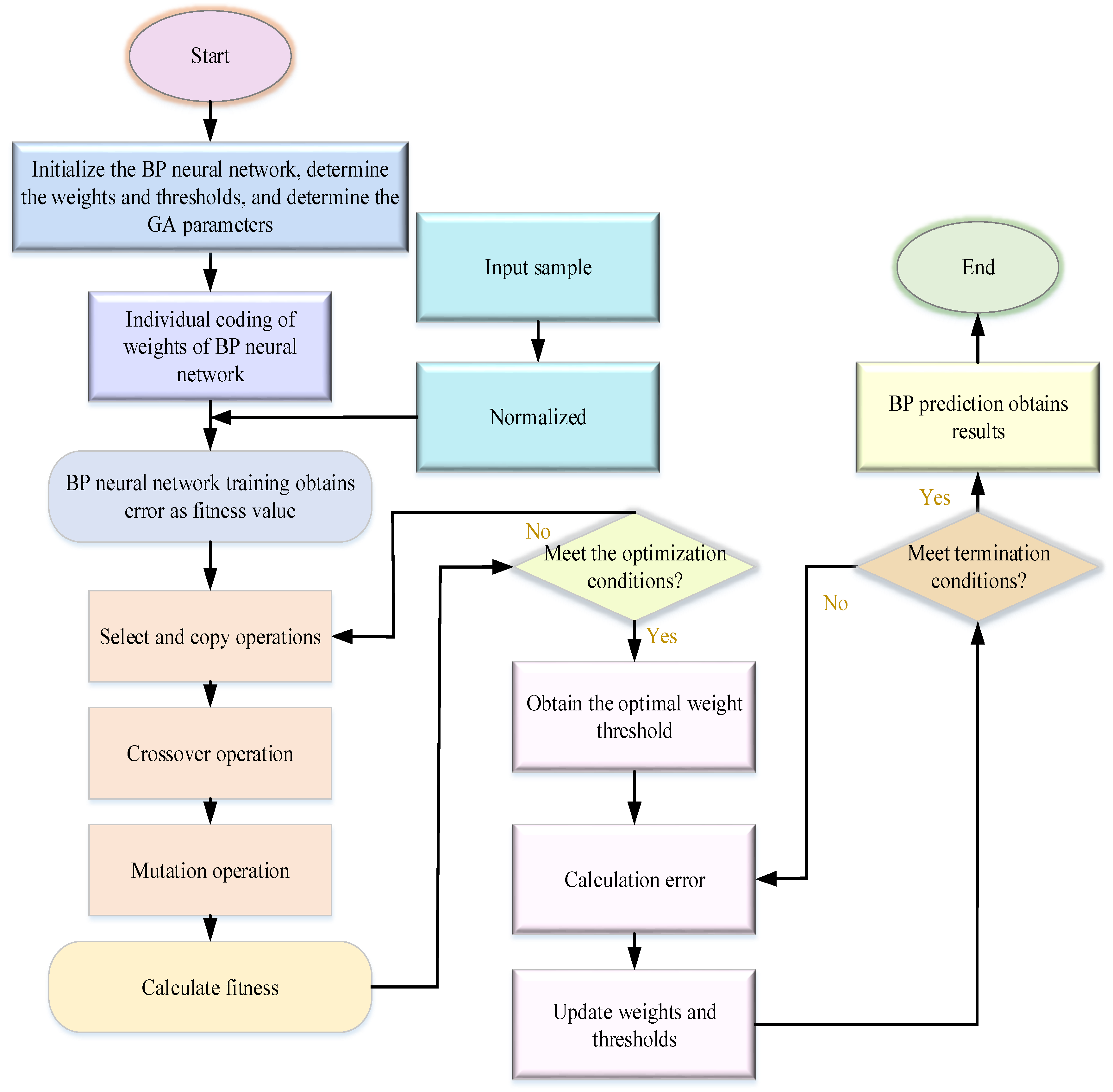
In Equations (17) and (18), , , and are the gene, the minimum , and maximum , respectively. represents a random number ∈[0, 1]. , , and mean the random number, iteration number, and the maximum number of evolutions, respectively. To sum up, the flow of the GA-optimized BPNN is shown in Figure 6.
2.4. Construction of the Air Quality–Meteorology Correlation Fusion Model Based on RF + BP + GA
Through the above explanation of the basic principles of RF and the improvement of BP through the GA, the two are combined to implement an air quality fusion model. The air quality–meteorology correlation fusion model based on RF + BP + GA is illustrated in Figure 7.
In Figure 7, the air quality–meteorology correlation fusion model based on RF + BP + GA first uses RF to extract air and meteorological quality features, mainly humidity and temperature. Here, it provides a training feature subset for the air quality–meteorology correlation fusion model. Second, the BPNN training model optimized with the GA is used to pre-train the feature subset to reduce the overfitting problem in the model training process and improve the training performance of the model. At last, the BPNN training model optimized with the GA is used to predict the AQI value. The RF + BP + GA fusion model reduces the dimension of the input features, reduces the influence of irrelevant factors on the training results, and realizes the optimization of the air quality–meteorology correlation fusion model.
2.5. The Role of Forests in Climate Regulation
The amount of carbon dioxide in forests varies between day and night, seasons, and weather conditions. Plants photosynthesize during the day, absorbing carbon dioxide from the air and releasing oxygen. At night, when photosynthesis stops and respiration begins. They take oxygen from the air and release carbon dioxide. Therefore, the percentage of carbon dioxide in the forest is different at night than during the day. Trees’ photosynthesis intensity is closely related to temperature. When the temperature is too low, photosynthesis slows down. If the temperature is high, photosynthesis is fast. When it gets too hot, photosynthesis stops again. Therefore, carbon dioxide demand is more or less different between seasons, weather conditions, high and low temperatures, and strong and weak photosynthesis. In short, carbon dioxide in the forest also decreases as the height of the forest increases. Moreover, at different times, it also changes between day and night, seasons, and weather conditions.
Forests act as carbon sinks, removing pollutants from the atmosphere, and are versatile tools to combat air pollution and mitigate climate change. Forests absorb a third of the carbon dioxide released by fossil fuels worldwide every year. Forests and climate are interdependent. On the one hand, a forest needs suitable environmental conditions as a plant community. Light, heat, water, and other conditions directly affect the geographical distribution range and spatial and temporal distribution pattern of various forest products and temperature changes. A dry or wet climate directly or indirectly affects the structure and function of the forest ecosystem. Therefore, if the climate changes, forest ecosystems will be affected. On the other hand, the forest itself can form a special microclimate. The forest changes the emissivity and thermal properties of the underlying surface. The forest climate is similar to the ocean’s, with gentle temperature variations in relatively wet forests and nearby areas. In general, the reflectance of the forest is only half that of the soil. Solar radiation passes through the atmosphere, reaches the surface, and is absorbed by the forest layer. The solar radiation occupies 30% of the land area and then is transferred to the atmosphere through long-wave radiation, latent heat release, and sensible heat transfer. Forests can be considered one of the heat reservoirs of the climate system. Forests partly affect precipitation, so forest destruction reduces the absorption of solar radiation and affects the water cycle. Large-scale forest changes may even affect global heat and water balances. As one of the components of the global climate system, forests stabilize the regional climate and thus play a role in stabilizing the global climate.
Forest carbon sinks are important for mitigating the effects of climate warming. However, under climate change, forests could easily become carbon sources rather than sinks. Natural disturbance mechanisms such as fire, pests, or drought can affect major forest functions, production, and stability. Applying the air quality–meteorology correlation model to forest ecosystem monitoring can provide data support for forest ecosystem management and facilitate the effective management of forest managers.
2.6. Experimental Software Environment Settings
This section uses the Spark framework of the Hadoop big data platform and sets three distributed frameworks. The operating system chooses Ubuntu 14.04 LTS. The software uses the crontab command in the Ubuntu system to implement the timing execution. In this experiment, the model execution task was set to be executed every 3 min. The JDK (Java Development Kit) version is JDK-7u80-Linux-x64, the Hadoop platform version is Hadoop-2.6, and the Spark version is 1.5.1.
3. Results and Discussion
3.1. Analysis of the Relationship between Air Quality and Meteorology
This section discusses the theory of the RF algorithm, expounds on the BPNN and related theories, and uses GA to optimize the prediction of the network weight and threshold of the BPNN. We sample the air quality of Xi’an from 24 to 30 June 2022, as the research object to analyze the impact of meteorological factors on air quality, such as temperature, humidity, and wind. The prediction results of the RF and BP–GA (Backpropagation–Genetic Algorithm) neural network algorithm in the air quality correlation model are analyzed. The changing trend of the AQI and meteorological conditions is described in Figure 8.
In Figure 8a, the changing law of AQI is consistent with the changing law of average temperature. The average temperature on 26 June 2022 was the lowest, the average temperature gradually decreased from 24 June 2022 to 25 June 2022, and the average temperature gradually increased from the 26 June 2022 to 30 June 2022. Therefore, there was a certain positive correlation between the average temperature and AQI. In Figure 8b, the relative humidity changed greatly from 25 June 2022 to 27 June 2022, averaging 52.33%. The relative humidity changed slightly for the rest of the time, averaging 31.75%. At the same time, the AQI value was relatively high when the relative humidity was low and relatively low when the relative humidity was high. It can be concluded that there is a certain negative correlation between relative humidity and AQI. In Figure 8c, the trend of wind level is relatively flat compared with AQI. From 24 June 2022 to 27 June 2022, the wind level changed the most, and the wind level on the other days remained at about level 2. When the wind level was high, the AQI value was relatively low. It can be inferred that there is a certain negative correlation between wind level and AQI. The difference between meteorological conditions and AQI values from 24 to 30 June 2022, is sketched in Table 3.
In Table 3, it can be seen from the value of AQI that the change in AQI value from 24 to 30 June 2022, is too large, and the data difference is 120. The minimum value of AQI is 46, and the maximum value of AQI is 166, which indicates moderate air-quality pollution, indicating that air-quality pollution has occurred in this area. Moreover, the maximum and minimum values of temperature, humidity, and wind meteorological factors in the region at the end of June were quite different, and the air quality in the region at the end of June was affected by meteorological conditions.
3.2. Analysis of the Prediction Results of the Air Quality–Meteorology Correlation Model Based on RF and BP–GA
The air quality–meteorology correlation model is constructed on the basis of RF and BP–GA. The AQI prediction results are demonstrated in Figure 9.
In Figure 9a, most of the predicted AQI values by the RF model are similar but lower than the actual AQI values. In Figure 9b, the predicted AQI values by the BP–GA model are close to but higher than the actual AQI values. Table 4 details the differences in the predicted numerical values of the air quality–meteorology correlation model of the different models.
Table 4 indicates that the output interval of the AQI value predicted by the RF model is [42.3, 168.29] compared with the AQI value predicted by the BP + GA model, which output interval is [47.23, 164.32] and which is closer to the actual predicted value of AQI. However, combined with the data shown in Figure 9, there is still a certain data gap between the RF model and the BP + GA model in predicting the AQI value. Therefore, this work fuses the RF and BP–GA models to jointly forecast AQI. The prediction results of the fusion model are shown in Figure 10.
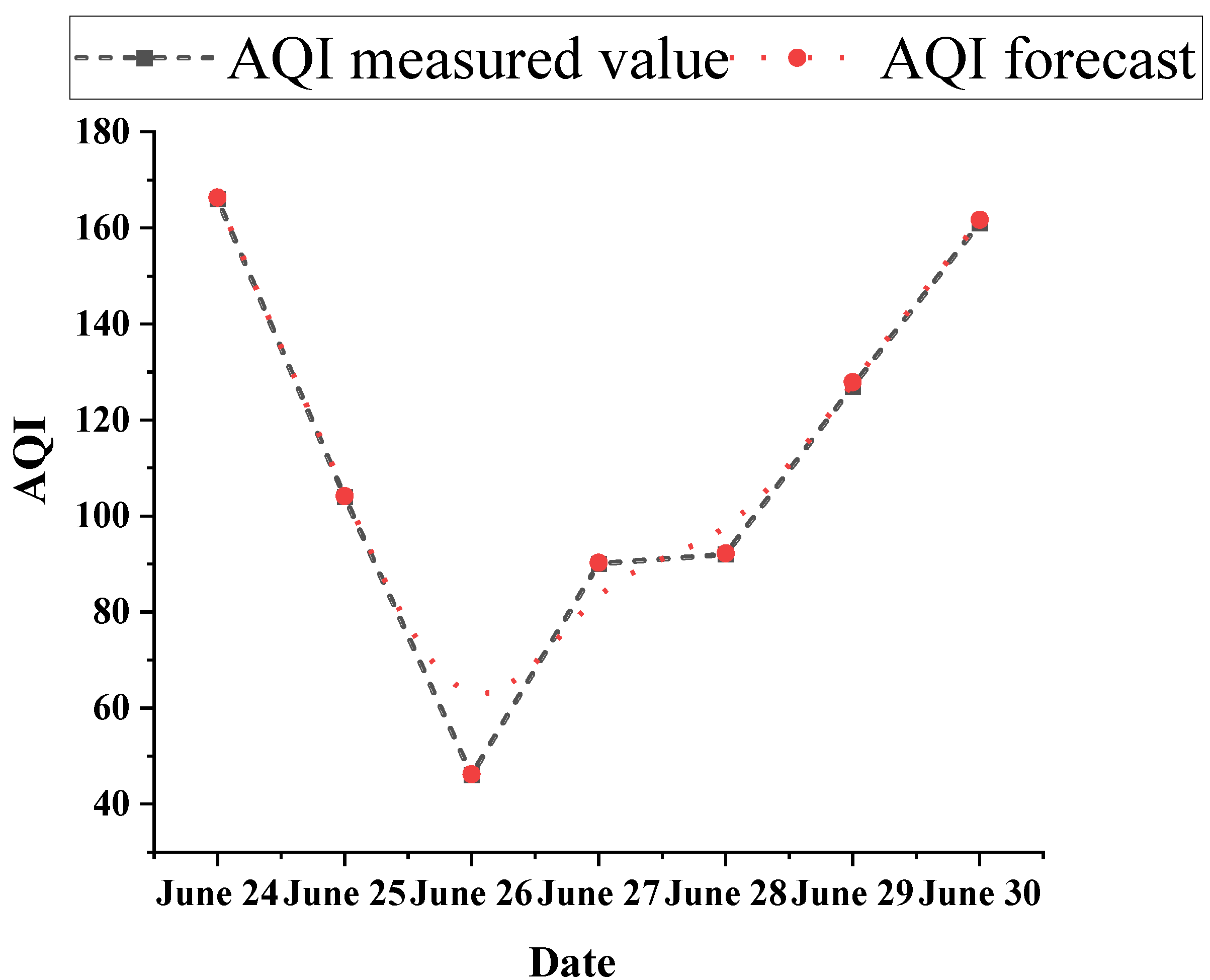
Clearly, the AQI predicted by the RF + BP + GA fusion-based air quality–meteorology correlation model coincides with the actual measurement, and the trend of the predicted and actual values are the same. Thus, the fitting effect of the RF + BP + GA fusion-based air quality–meteorology correlation model is the best, achieving a complete fitting to accurately forecast the AQI. The differences in the prediction values of the RF + BP + GA fusion-based air quality–meteorology correlation model are indicated in Table 5.
Table 5 describes that the data gap between the AQI value of the RF + BP + GA fusion model and the AQI value of the actual air quality meteorology is [0.23, 0.32], which is very small. In summary, the prediction results of the RF-based and BP–GA-based air quality–meteorology correlation model are slightly lower and higher than the real values. The prediction results of the RF + BP + GA fusion-based air quality–meteorology correlation model are closest to the real values. Thus, fusing RF and BP–GA to build the air quality–meteorology correlation model can best predict the AQI.
3.3. Discussion
The air quality–meteorology correlation model uses a fusion model of RF + BP + GA to predict air quality. Through analyzing the air quality and meteorological conditions in Xi’an from 24 to 30 June 2022, it is found that there is a certain positive correlation between average temperature and AQI, while there is a certain negative correlation between relative humidity and AQI. This result is consistent with the research results of Kais et al. [44], who used RF to evaluate and predict the air quality of 113 environmental protection cities in China from 2014 to 2016. The survey results found a correlation between air quality levels and AQI values. Furthermore, the AQI value predicted by the RF + BP + GA model is basically coincident with the AQI value obtained with the actual measurement. The RF + BP + GA model has the best fitting effect among the air quality–meteorology correlation models, basically achieves complete fitting, and can accurately predict the AQI value of air quality. Jiang et al. [45] established the fusion model of the limit gradient lifting algorithm + BP + autoregressive moving average model to jointly predict the air quality in Changping District, Beijing. They found that the prediction effect of the proposed model was more accurate than the air quality prediction of a single limit gradient lifting algorithm, BPNN, or autoregressive moving average model. The results demonstrate the prediction effect of the fusion model in this work and show that the prediction effect of the fusion model is better than that of a single algorithm in predicting air quality. When Qiao et al. [46] used BPNN and RF to predict the concentration of air pollutants, they found that the AQI accuracy of BP + RF prediction was about 87%. However, comparing the AQI values used here reflects our model’s better prediction accuracy. It is found that the AQI value predicted by the RF + BP + GA model basically coincides with the AQI value obtained with the actual measurement, so the AQI value predicted by the RF + BP + GA model achieves a good prediction accuracy, which proves the effectiveness of the proposed RF + BP + GA fusion-based air quality–meteorology correlation model.
4. Conclusions
The air quality was collected in Xi’an from 24 to 30 June 2022. Following an analysis of the changing trends of air quality, AQI, and input variables, this work takes meteorological factors—relative humidity, wind level, and average temperature—as the input variables for the air quality–meteorology correlation model. Meanwhile, it introduces the AQI as the output variable. As a result, a BPNN model optimized with RF and GA is proposed to forecast the air quality in Xi’an. The relationship between temperature, humidity, wind level, and air quality is analyzed. The influence of climate change on the forest ecosystem is illustrated, and the interaction between the air quality–climate correlation model and the forest ecosystem is explored. The prediction results of RF-based, BP–GA-based, and RF + BP + GA fusion-based air quality–meteorology correlation models are analyzed and compared. The results show a positive correlation between average temperature and AQI, a negative correlation between relative humidity and AQI, and a negative correlation between wind level and AQI. The predicted AQI values by the RF-based and BP–GA models are slightly lower and higher than the actual AQI values, respectively. The fitting effect of the RF + BP + GA fusion-based air quality–meteorology correlation model is the best, and the complete fitting is basically realized. The prediction error of the proposed RF + BP + GA model for AQI is not more than 0.32, which shows a good fitting effect with the actual value. The fusion air quality–meteorology correlation model can accurately forecast the AQI. Inevitably, meteorological conditions’ seasonal and interannual fluctuations impact air quality. However, even in short-term or long-term adverse conditions, it is always imperative to focus on the long term and make steady progress following scientific and accurate pollution control principles. Forests and climate are interdependent. Forests act as carbon sinks, removing pollutants from the atmosphere and serving as a multifunctional tool to combat air pollution and mitigate climate change.
The findings provide research references for predicting the AQI using an air quality–meteorology correlation model and data support for analyzing air quality problems. The ecological relationship between climate and forest is expounded in detail, and the change and development of forest ecosystems under the air quality–climate correlation model are studied, which provides a reference for research on the interaction between climate and forest ecosystems. Last but not least, there are still some shortcomings of this work. Firstly, the sample size is too small. Secondly, although the BPNN is optimized, the optimization results of other machine-learning methods on the neural network are not compared. In addition, this work uses the air quality–meteorology correlation model of Xi’an in June 2022 for prediction analysis. There was a high temperature during this period, and the changes in other meteorological factors caused by these high temperatures are unknown. It is hoped that the impact of meteorological factors on air quality changes can be comprehensively considered in future research. The amount of training data can also be expanded, such as meteorological changes in air quality in Xi’an within one year in 2021. Various algorithms can be considered to optimize the neural network, and the optimization effects of other machine-learning algorithms on the neural network can be compared and analyzed.
Author Contributions
Each author made significant individual contributions to this manuscript. R.L.: methodology, data analysis, and writing; L.P.: data analysis, writing—reviewing and editing; Y.Y.: article review and intellectual concept of the article; Y.G.: research and investigation; B.G.: consulting materials and references; F.L.: article review and intellectual concept of the article; L.W.: consulting materials and references. All authors have read and agreed to the published version of the manuscript.
Funding
Natural Science Basic Research Program of Shaanxi, Numerical Simulation of Atmospheric Fine Particles on Guanzhong Urban Agglomeration, 2021JQ-975; Natural Science Basic Research Program of Shaanxi, Research on Strong Convective Weather Forecast and Warning Method Using Meteorological Data and Artificial Intelligence Technology, 2022JQ-296.
Conflicts of Interest
The authors declare that the research was conducted in the absence of any commercial or financial relationships that could be construed as potential conflict of interest.
References
- Zhao, S.; Jiang, Y.; Wang, S. Innovation stages, knowledge spillover, and green economy development: Moderating role of absorptive capacity and environmental regulation. Environ. Sci. Pollut. Res. 2019, 26, 25312–25325. [Google Scholar] [CrossRef] [PubMed]
- Chen, Y.; Zhang, L.; Henze, D.K.; Zhao, Y.; Lu, X.; Winiwarter, W.; Guo, Y.; Liu, X. Interannual variation of reactive nitrogen emissions and their impacts on PM2.5 air pollution in China during 2005–2015. Environ. Res. Lett. 2021, 16, 125004. [Google Scholar] [CrossRef]
- Chen, D.; Liang, D.; Li, L.; Guo, X.; Lang, J.; Zhou, Y. The temporal and spatial changes of ship-contributed PM2.5 due to the inter-annual meteorological variation in Yangtze river delta, China. Atmosphere 2021, 12, 722. [Google Scholar] [CrossRef]
- Liu, Y.; Failler, P.; Liu, Z. Impact of Environmental Regulations on Energy Efficiency: A Case Study of China’s Air Pollution Prevention and Control Action Plan. Sustainability 2022, 14, 3168. [Google Scholar] [CrossRef]
- Zhang, Z.; Zhang, J.; Feng, Y. Assessment of the Carbon Emission Reduction Effect of the Air Pollution Prevention and Control Action Plan in China. Int. J. Environ. Res. Public Health 2021, 18, 13307. [Google Scholar] [CrossRef] [PubMed]
- Yang, Q.; Gao, D.; Song, D.; Li, Y. Environmental regulation, pollution reduction and green innovation: The case of the Chinese Water Ecological Civilization City Pilot policy. Econ. Syst. 2021, 45, 100911. [Google Scholar] [CrossRef]
- Akinwumiju, A.S.; Ajisafe, T.; Adelodun, A.A. Airborne particulate matter pollution in akure metro city, southwestern Nigeria, west Africa: Attribution and meteorological influence. J. Geovisualization Spat. Anal. 2021, 5, 1–17. [Google Scholar] [CrossRef]
- Li, H.; Deng, J.; Yuan, S.; Feng, P.; Arachchige, D. Monitoring and Identifying Wind Turbine Generator Bearing Faults using Deep Belief Network and EWMA Control Charts. Front. Energy Res. 2021, 9, 799039. [Google Scholar] [CrossRef]
- He, Y.; Kusiak, A. Performance assessment of wind turbines: Data-derived quantitative metrics. IEEE Trans. Sustain. Energy 2017, 9, 65–73. [Google Scholar] [CrossRef]
- Li, H. Short-term Wind Power Prediction via Spatial Temporal Analysis and Deep Residual Networks. Front. Energy Res. 2022, 10, 920407. [Google Scholar] [CrossRef]
- Li, H. SCADA Data based Wind Power Interval Prediction using LUBE-based Deep Residual Networks. Front. Energy Res. 2022, 10, 920837. [Google Scholar] [CrossRef]
- Subudhi, A.; Dash, M.; Sabut, S. Automated segmentation and classification of brain stroke using expectation-maximization and random forest classifier. Biocybern. Biomed. Eng. 2020, 40, 277–289. [Google Scholar] [CrossRef]
- Brieuc, M.S.O.; Waters, C.D.; Drinan, D.P.; Naish, K.A. A practical introduction to Random Forest for genetic association studies in ecology and evolution. Mol. Ecol. Resour. 2018, 18, 755–766. [Google Scholar] [CrossRef] [PubMed]
- Wang, X.; Yu, B.; Ma, A.; Chen, C.; Liu, B.; Ma, Q. Protein–protein interaction sites prediction by ensemble random forests with synthetic minority oversampling technique. Bioinformatics 2019, 35, 2395–2402. [Google Scholar] [CrossRef] [PubMed]
- Lolli, S.; Chen, Y.C.; Wang, S.H.; Vivone, G. Impact of meteorological conditions and air pollution on COVID-19 pandemic transmission in Italy. Sci. Rep. 2020, 10, 16213. [Google Scholar] [CrossRef] [PubMed]
- Ceylan, Z. Insights into the relationship between weather parameters and COVID-19 outbreak in Lombardy, Italy. Int. J. Healthc. Manag. 2021, 14, 255–263. [Google Scholar] [CrossRef]
- Zhou, X.; Tang, X.; Zhang, R. Impact of green finance on economic development and environmental quality: A study based on provincial panel data from China. Environ. Sci. Pollut. Res. 2020, 27, 19915–19932. [Google Scholar] [CrossRef]
- Gan, T.; Yang, H.; Liang, W.; Liao, X. Do economic development and population agglomeration inevitably aggravate haze pollution in China? New evidence from spatial econometric analysis. Environ. Sci. Pollut. Res. 2021, 28, 5063–5079. [Google Scholar] [CrossRef]
- Shahriar, S.A.; Kayes, I.; Hasan, K.; Hasan, M.; Islam, R.; Awang, N.R.; Hamzah, Z.; Rak, A.E.; Salam, M.A. Potential of Arima-ann, Arima-SVM, dt and catboost for atmospheric PM 2.5 forecasting in bangladesh. Atmosphere 2021, 12, 100. [Google Scholar] [CrossRef]
- Gocheva-Ilieva, S.; Ivanov, A.; Stoimenova-Minova, M. Prediction of daily mean PM10 concentrations using random forest, CART Ensemble and Bagging Stacked by MARS. Sustainability 2022, 14, 798. [Google Scholar] [CrossRef]
- Menéndez García, L.A.; Menéndez Fernández, M.; Sokoła-Szewioła, V.; Álvarez de Prado, L.; Ortiz Marqués, A.; Fernández López, D.; Bernardo Sánchez, A. A Method of Pruning and Random Replacing of Known Values for Comparing Missing Data Imputation Models for Incomplete Air Quality Time Series. Appl. Sci. 2022, 12, 6465. [Google Scholar] [CrossRef]
- Liu, B.; Zhao, Q.; Jin, Y.; Li, C. Application of combined model of stepwise regression analysis and artificial neural network in data calibration of miniature air quality detector. Sci. Rep. 2021, 11, 3247. [Google Scholar] [CrossRef]
- Li, G.; Wang, H.; Zhang, S.; Xin, J.; Liu, H. Recurrent neural networks based photovoltaic power forecasting approach. Energies 2019, 12, 2538. [Google Scholar] [CrossRef] [Green Version]
- Ogheneovo, E.E.; Nlerum, P.A. Iterative dichotomizer 3 (ID3) decision tree: A machine learning algorithm for data classification and predictive analysis. Int. J. Adv. Eng. Res. Sci. 2020, 7, 514–521. [Google Scholar] [CrossRef]
- Althuwaynee, O.F.; Balogun, A.L.; Al Madhoun, W. Air pollution hazard assessment using decision tree algorithms and bivariate probability cluster polar function: Evaluating inter-correlation clusters of PM10 and other air pollutants. GIScience Remote Sens. 2020, 57, 207–226. [Google Scholar] [CrossRef]
- Singh, V.; Poonia, R.C.; Kumar, S.; Dass, P.; Agarwal, P.; Bhatnagar, V.; Raja, L. Prediction of COVID-19 corona virus pandemic based on time series data using Support Vector Machine. J. Discret. Math. Sci. Cryptogr. 2020, 23, 1583–1597. [Google Scholar] [CrossRef]
- Eldakhly, N.M.; Aboul-Ela, M.; Abdalla, A. A novel approach of weighted support vector machine with applied chance theory for forecasting air pollution phenomenon in Egypt. Int. J. Comput. Intell. Appl. 2018, 17, 1850001. [Google Scholar] [CrossRef]
- Jiang, X.; Zhang, X.; Zhang, Y. Establishment and optimization of sensor fault identification model based on classification and regression tree and particle swarm optimization. Mater. Res. Express 2021, 8, 085703. [Google Scholar] [CrossRef]
- Bai, C.; Sarkis, J. Green supplier development: Analytical evaluation using rough set theory. J. Clean. Prod. 2010, 18, 1200–1210. [Google Scholar] [CrossRef]
- Kalajdjieski, J.; Zdravevski, E.; Corizzo, R.; Lameski, P.; Kalajdziski, S.; Pires, I.M.; Garcia, N.M.; Trajkovik, V. Air pollution prediction with multi-modal data and deep neural networks. Remote Sens. 2020, 12, 4142. [Google Scholar] [CrossRef]
- Shanahan, J.; Wall, T. ‘Fight the reds, support the blue’: Blue Lives Matter and the US counter-subversive tradition. Race Cl. 2021, 63, 70–90. [Google Scholar] [CrossRef]
- Navinya, C.D.; Vinoj, V.; Pandey, S.K. Evaluation of PM2.5 surface concentrations simulated by NASA’s MERRA version 2 aerosol reanalysis over India and its relation to the air quality index. Aerosol Air Qual. Res. 2020, 20, 1329–1339. [Google Scholar] [CrossRef] [Green Version]
- Hu, F.; Guo, Y. Impacts of electricity generation on air pollution: Evidence from data on air quality index and six criteria pollutants. SN Appl. Sci. 2021, 3, 4. [Google Scholar] [CrossRef]
- Song, Z.; Deng, Q.; Ren, Z. Correlation and principal component regression analysis for studying air quality and meteorological elements in Wuhan, China. Environ. Prog. Sustain. Energy 2020, 39, 13278. [Google Scholar] [CrossRef]
- Fu, D.; Shi, X.; Xing, Y.; Wang, P.; Li, H.; Li, B.; Lu, L.; Thapa, S.; Yabo, S.; Qi, H.; et al. Contributions of extremely unfavorable meteorology and coal-heating boiler control to air quality in December 2019 over Harbin, China. Atmos. Pollut. Res. 2021, 12, 101217. [Google Scholar] [CrossRef]
- Jia, Y.; Jin, S.; Savi, P.; Yan, Q.; Li, W. Modeling and theoretical analysis of GNSS-R soil moisture retrieval based on the random forest and support vector machine learning approach. Remote Sens. 2020, 12, 3679. [Google Scholar] [CrossRef]
- Slobbe, L.C.J.; Füssenich, K.; Wong, A. Estimating disease prevalence from drug utilization data using the Random Forest algorithm. Eur. J. Public Health 2019, 29, 615–621. [Google Scholar] [CrossRef]
- Yu, Z.; Shi, X.; Qiu, X.; Zhou, J.; Chen, X. Optimization of postblast ore boundary determination using a novel sine cosine algorithm-based random forest technique and Monte Carlo simulation. Eng. Optim. 2021, 53, 1467–1482. [Google Scholar] [CrossRef]
- Li, T.; Sun, J.; Wang, L. An intelligent optimization method of motion management system based on BP neural network. Neural Comput. Appl. 2021, 33, 707–722. [Google Scholar] [CrossRef]
- Yuan, R.; Lv, Y.; Kong, Q. Percussion-based bolt looseness monitoring using intrinsic multiscale entropy analysis and BP neural network. Smart Mater. Struct. 2019, 28, 125001. [Google Scholar] [CrossRef]
- Han, J.X.; Ma, M.Y.; Wang, K. Product modeling design based on genetic algorithm and BP neural network. Neural Comput. Appl. 2021, 33, 4111–4117. [Google Scholar] [CrossRef]
- Zhang, D.; Li, W.; Wu, X.; Lv, X. Application of simulated annealing genetic algorithm-optimized back propagation (BP) neural network in fault diagnosis. Int. J. Model. Simul. Sci. Comput. 2019, 10, 1950024. [Google Scholar] [CrossRef]
- Soepangkat, B.O.P.; Pramujati, B.; Effendi, M.K. Multi-objective optimization in drilling kevlar fiber reinforced polymer using grey fuzzy analysis and Backpropagation Neural Network–Genetic Algorithm (BPNN–GA) Approaches. Int. J. Precis. Eng. Manuf. 2019, 20, 593–607. [Google Scholar] [CrossRef]
- Kais, K.; Gołaś, M.; Suchocka, M. Awareness of Air Pollution and Ecosystem Services Provided by Trees: The Case Study of Warsaw City. Sustainability 2021, 13, 10611. [Google Scholar] [CrossRef]
- Jiang, W.; Zhu, G.; Shen, Y. An Empirical Mode Decomposition Fuzzy Forecast Model for Air Quality. Entropy 2022, 24, 1803. [Google Scholar] [CrossRef]
- Qiao, D.; Yao, J.; Zhang, J. Short-term air quality forecasting model based on hybrid RF-IACA-BPNN algorithm. Environ. Sci. Pollut. Res. 2022, 29, 39164–39181. [Google Scholar] [CrossRef]
Figure 1.
Changes in AQI index value in Xi’an from 24 to 30 June 2022.

Figure 2.
Basic principles of RF (A, B, C represent different results of different decision tree prediction classifications).
Figure 2.
Basic principles of RF (A, B, C represent different results of different decision tree prediction classifications).

Figure 3.
The importance of sample features in RF training.

Figure 4.
The connection structure between BPNN neurons.

Figure 5.
The initialization operation, exchange operation, and mutation operation processes of GA.

Figure 6.
The flow of GA-optimized BPNN.

Figure 7.
The air quality–meteorology correlation fusion model based on RF + BP + GA.

Figure 8.
The changing trend of AQI and meteorological conditions: (a) is the trend of temperature and AQI; (b) is the trend of relative humidity and AQI, and (c) indicates the trend of wind level and AQI.
Figure 8.
The changing trend of AQI and meteorological conditions: (a) is the trend of temperature and AQI; (b) is the trend of relative humidity and AQI, and (c) indicates the trend of wind level and AQI.

Figure 9.
The prediction results of the air quality–meteorology correlation model: (a) is the prediction results of the RF model; (b) is the prediction results of the BP–GA model.
Figure 9.
The prediction results of the air quality–meteorology correlation model: (a) is the prediction results of the RF model; (b) is the prediction results of the BP–GA model.

Figure 10.
Prediction results of the RF + BP + GA fusion-based air quality–meteorology correlation model.
Figure 10.
Prediction results of the RF + BP + GA fusion-based air quality–meteorology correlation model.


Table 1.
The applicable range of different evaluation indices.
| Evaluation Index | Evaluation Scope | Applicable Range |
|---|---|---|
| AQI | It can quantitatively describe air quality. | AQI (Air Quality Index). Each pollutant is converted into AQI during the evaluation according to different target concentration limits. |
| API | It is a quantitative index to evaluate the quality of air. | Status and trends of short-term air quality in cities. |
| ORAQI | It mainly evaluates sulfur dioxide (SO2), nitrogen dioxide (NO2), carbon monoxide (CO), Total Suspended Particle (TSP), and oxidants. | Annual change in air quality in a city or region. |
| EVI | It mainly uses SO2, CO, TSP, and oxidants as indicators. | Changes in high-concentration pollution in a day. |
| PSI | It mainly evaluates SO2, NO2, CO, TSP, and oxidants. | Changes in urban air pollution. |
Table 2.
Steps of RF algorithm flow.
| Start: | ||
|---|---|---|
| Input: | Original sample set . | Test sample . |
| Sampling: | The original data is sampled with the Bagging algorithm. | Training subset . |
| Data set: | Select training subset as the dataset of the th DT. | Data set. |
| Calculate all node attributes of information gain: | Select all attributes of the node. | Calculate the information gain index of attributes. |
| DT splitting: | Select the attribute with the largest information gain as the classification node. | Obtain DTs. |
| Output: | is input into the DT . | Output classification results. |
| End: |
Table 3.
The difference between meteorological conditions and AQI values from 24 to 30 June 2022.
| Meteorological Conditions | Maximum | Minimum | Mean | The Maximum Value of AQI | The Minimum Value of AQI |
|---|---|---|---|---|---|
| Temperature | 36 | 25 | 30 | 166 | 46 |
| Humidity | 0.77 | 0.27 | 0.41 | 166 | 46 |
| Wind | 4.5 | 1 | 2.7 | 166 | 46 |
Table 4.
The differences in the predicted numerical values of the air quality–meteorology correlation model of different models.
Table 4.
The differences in the predicted numerical values of the air quality–meteorology correlation model of different models.
| Predicted Training Model | RF Model | BP + GA Model |
|---|---|---|
| The maximum value of AQI | 166 | 166 |
| The maximum predicted value of AQI | 168.29 | 164.32 |
| The minimum value of AQI | 46 | 46 |
| The minimum predicted value of AQI | 42.3 | 47.23 |
Table 5.
The differences in prediction values of the RF + BP + GA fusion-based air quality–meteorology correlation model.
Table 5.
The differences in prediction values of the RF + BP + GA fusion-based air quality–meteorology correlation model.
| RF + BP + GA Prediction Training Model | Numerical |
|---|---|
| The maximum value of AQI | 166 |
| The maximum predicted value of AQI | 166.32 |
| The minimum value of AQI | 46 |
| The minimum predicted value of AQI | 46.23 |
Disclaimer/Publisher’s Note: The statements, opinions and data contained in all publications are solely those of the individual author(s) and contributor(s) and not of MDPI and/or the editor(s). MDPI and/or the editor(s) disclaim responsibility for any injury to people or property resulting from any ideas, methods, instructions or products referred to in the content. |
© 2023 by the authors. Licensee MDPI, Basel, Switzerland. This article is an open access article distributed under the terms and conditions of the Creative Commons Attribution (CC BY) license (https://creativecommons.org/licenses/by/4.0/).
Share and Cite
MDPI and ACS Style
Liu, R.; Pang, L.; Yang, Y.; Gao, Y.; Gao, B.; Liu, F.; Wang, L. Air Quality—Meteorology Correlation Modeling Using Random Forest and Neural Network. Sustainability 2023, 15, 4531. https://doi.org/10.3390/su15054531
AMA Style
Liu R, Pang L, Yang Y, Gao Y, Gao B, Liu F, Wang L. Air Quality—Meteorology Correlation Modeling Using Random Forest and Neural Network. Sustainability. 2023; 15(5):4531. https://doi.org/10.3390/su15054531
Chicago/Turabian StyleLiu, Ruifang, Lixia Pang, Yidian Yang, Yuxing Gao, Bei Gao, Feng Liu, and Li Wang. 2023. "Air Quality—Meteorology Correlation Modeling Using Random Forest and Neural Network" Sustainability 15, no. 5: 4531. https://doi.org/10.3390/su15054531
Note that from the first issue of 2016, this journal uses article numbers instead of page numbers. See further details here.